In the previous post a lot of things have happened and went sideways, making the whole process a lot slower than it needed to be. Acceptable outcome, since many moving parts had to work before something could actually happen.
This time around we are a bit better off and can afford to plan a bit ahead and test things out with Godot beforehand.
The goal is to make the overall scene a bit more presentable. While originally I wanted to proceed with light and shadow implementations, eventually decided against it. The reason is that there is a more fundamental concept in graphics that is much more valuable.
Textures
Textures are a simple concept, brilliantly utilized in multiple ways. A chunk of memory organized into an array (1D texture), a matrix (2D texture) or 3D. A texture can be used to wrap an image around an object, define normals for the object, motion vectors, material properties and so on. They are fundamental for shadow algorithms, light baking and complex material properties.
To demonstrate how massively they can improve the visual experience observe the below comparison.
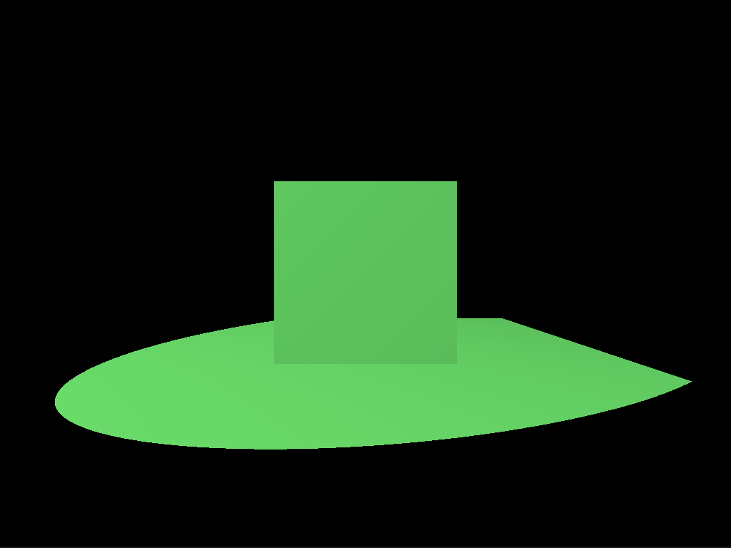
Previous state
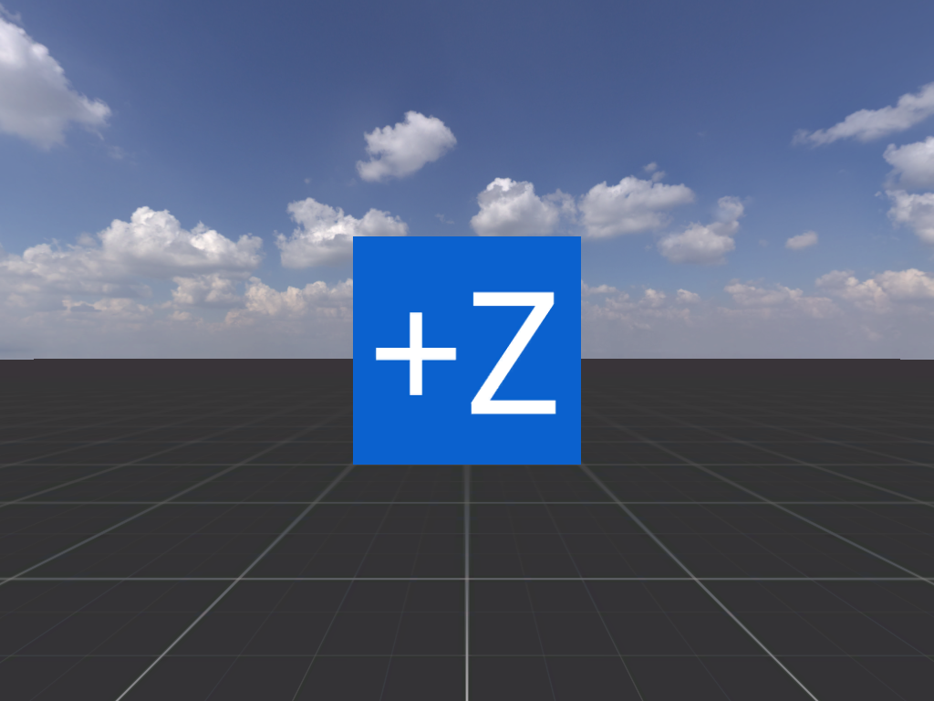
Just a few textures
Before we had a light which produced a green .. err .. glow I suppose. Now, the light has been removed and a texture was added to the ground plane, the cube and the sky. The absence of shadows makes the image a bit unnerving, but this is all we will need.
The only other thing needed again was a simple Godot spatial shader which circumvented basically all of Godot’s shading and lightning system ensuring that the only thing used for “coloring” a pixel was just a texture.
shader_type spatial;

render_mode unshaded;

uniform sampler2D plane_texture;
uniform vec2 uv_scale;

void vertex() {
	UV = UV * uv_scale;
}

void fragment() {
	vec3 sample = texture(plane_texture, UV).rgb;
	// force SRGB color
	ALBEDO = mix(pow((sample + vec3(0.055)) * (1.0 / (1.0 + 0.055)), vec3(2.4)), sample * (1.0 / 12.92), lessThan(sample,vec3(0.04045)));
}
The only “hack” that needed to be added was forcing the sRGB color space. Not entirely sure what that piece of code does, less so why, but seems to produce the expected result. Without it, the textures will not appear as they should and would have this washed out appearance to them.
Note that this little “hack” has been resolved since Part 3. In short the hack is incorrect, but you can ignore it for this post.
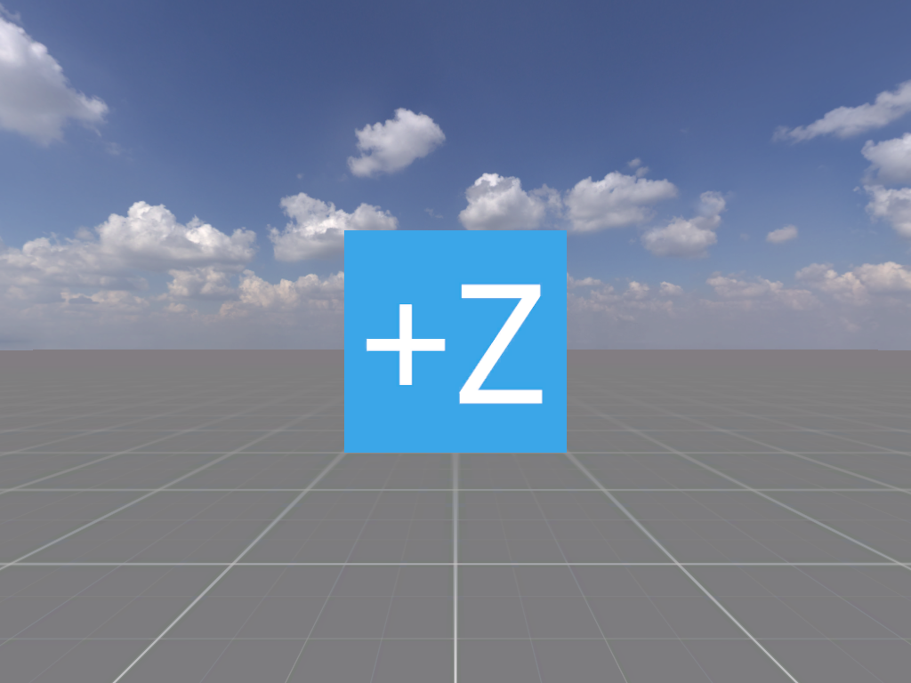
Without forced sRGB
This way, hopefully, we can relatively easily reproduce the results.
Sources
All textures are open source under the CCO 1.0 Universal license. You can use them for free, for commercial products as well, without any restrictions. Attributions are not required, but it is the least we can do to the artists/original sources.
The skybox is Kloofendal 48d Partly Cloudy (Pure Sky), from Poly Haven. Extremely high quality textures, for completely free!
The ground texture is taken from the Prototype Textures pack.
The cube texture was made by hand, but you may use it under the CCO 1.0 Universal license as well.
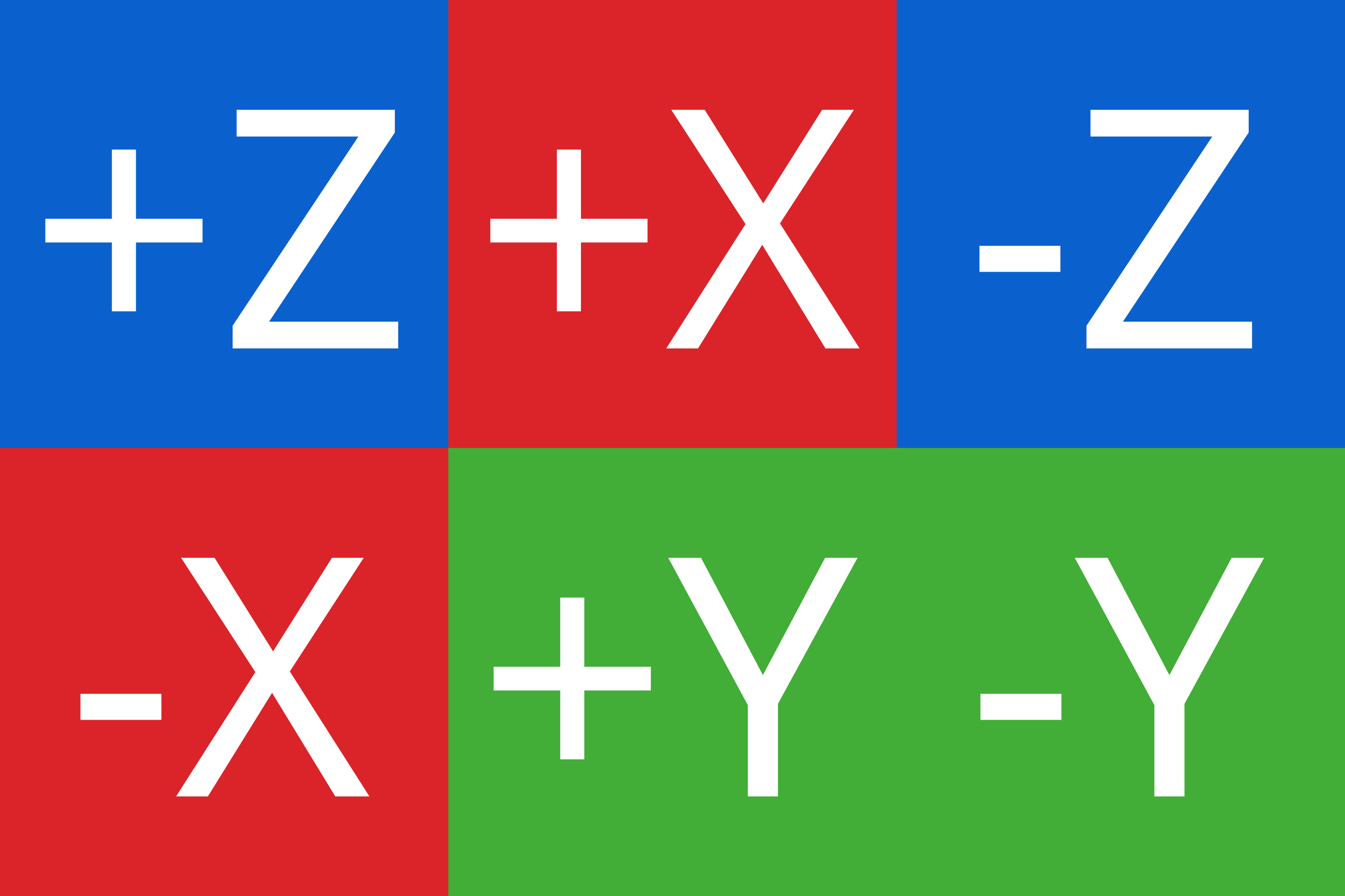
Cube texture
The following posts were invaluable in understanding what the basic concepts were and how one should think about them:
We will walk the same road, but only focusing on higher level abstractions and understanding.
The process
First, the light and any related code has been removed, and the fragment shader now simply returns a 20% grey color for any pixel. The plane was scaled to be 100x100 meters big and with this, the basic setup of our example scene has been achieved.
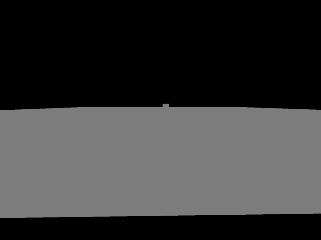
Scene
Next a simplest 2x2 texture was made to be used for the plane of the format:
green, blue
blue, green
This texture is repeated 50 times for the plane, resulting in a checkerboard pattern, where each rectangle is exactly a meter wide/tall. Observe below how the 2x2 cube is exactly a green and blue rectangle wide.
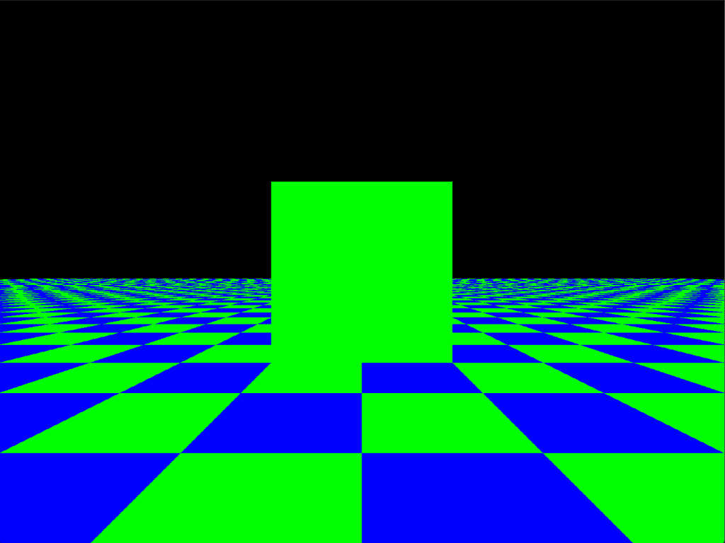
Checkerboard
These scales are very important, especially in such barren scenes, as they act as a reference for scale and orientation.
One thing that surprised me is that a texture and a sampler are special resources which cannot be handled as simple uniforms with WebGPU.
Initially, this was what I wanted to do:
struct Entity {
    world: mat4x4f,
    normal: mat3x3f,
    texture_sampler: sampler,
    texture: texture_2d<f32>,
}

@group(1)
@binding(0)
var<uniform> entity: Entity;
This though is simply not possible, because a texture and the sampler is a different type of resource, and even though it doesn’t change for a draw call (hence I thought it could be a uniform), it must be bound separately.
struct Entity {
    world: mat4x4f,
    normal: mat3x3f,
}

@group(1)
@binding(0)
var<uniform> entity: Entity;

@group(2)
@binding(0)
var texture_sampler: sampler;

@group(2)
@binding(1)
var texture: texture_2d<f32>;
Why exactly this may be is not clear. Perhaps because there are specialized internal representations and/or specific hardware elements which the GPU handles? A texture sampler is a built-in hardware component as it has to be extremely fast, similarly a texture is stored in GPU memory in a way that accelerates its access.
For example a simple 4x4 matrix like this:
i\j 0 1 2 3
0   a b c d
1   e f g h
2   i j k l
3   m n o p
In the most common, row major sequential memory layout format would look like this:
a b c d
e f g h
i j k l
m n o p
For demonstration purposes a line break was inserted at the end of each row. In practice this would just be a continuous piece of memory.
a b c d e f g h i j k l m n o p
This layout is very good for iterating the rows of the matrix very fast, because by loading a line into memory, a number of following elements will be loaded into the cache as well.
Textures though aren’t accessed in a sequential manner. A sampler has to be able to access the neighboring texels at a given coordinate very fast. A texel is a pixel of a texture. Instead of a sequential memory layout a Z-order curve is used.
Using Z-order curve memory layout the above matrix would look like this in memory:
a b e f c d g h i j m n k l o p
More on GPU cache locality can be found at Gpu cache hierarchy.
Loading the plane texture
You would think that just loading a PNG should be easy right? It is a just a simple file format that has been around forever. Tried loading the texture:
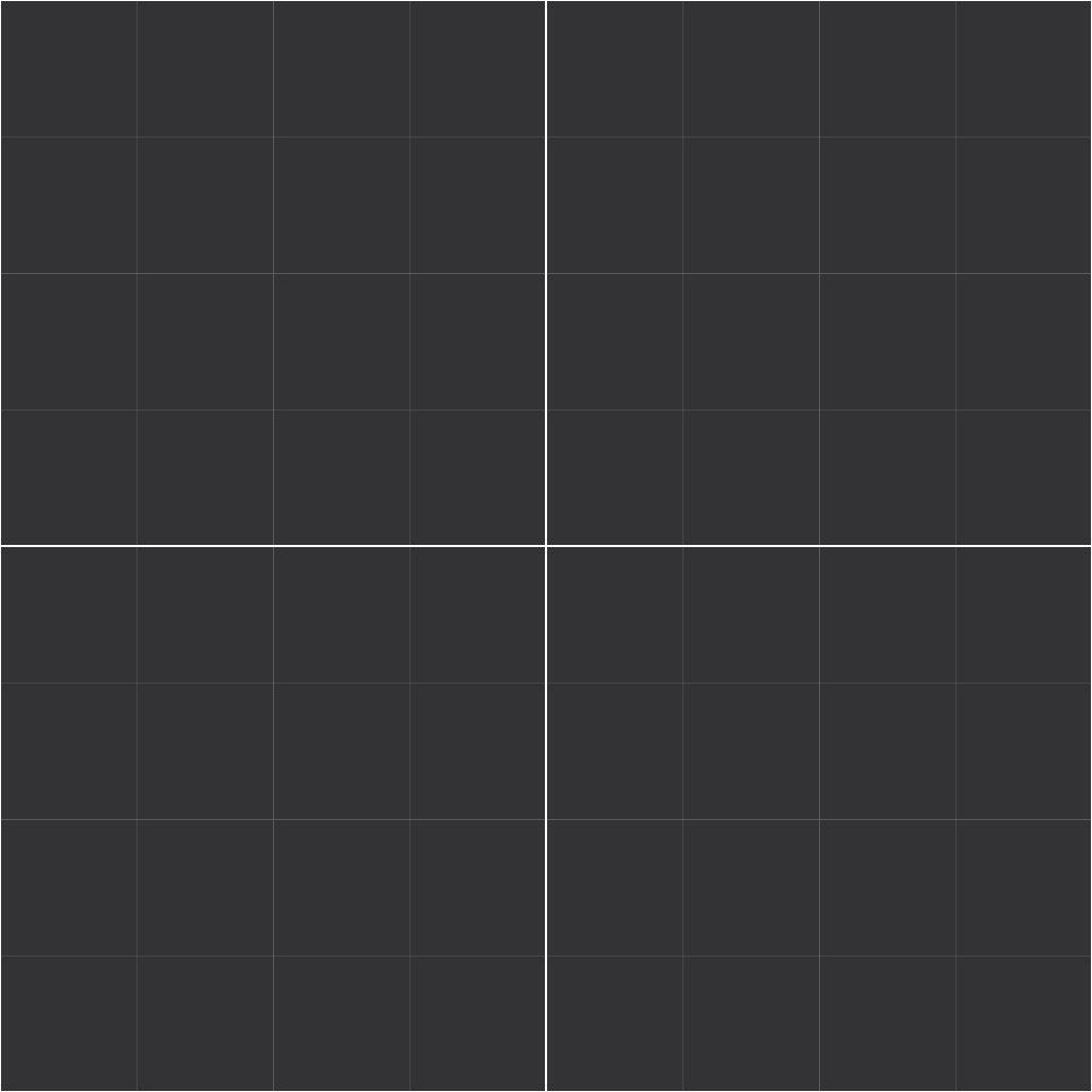
Plane texture
with the png rust library. It loaded, but something didn’t seem right, WebGPU would not accept it. Tried loading the wgpu logo, following the wgpu bunnymark example and that worked.

Wgpu logo
If I were to open the two textures with Krita it would say they have the format: RGB/Alpha (8-bit integer/channel), using the sRGB-elle-V2-srgbtrc.icc profile. On the other hand, when they were to be opened with Zed, for the texture_01.png it would be 3 channels 24 bits per pixel, for the logo.png 4 channels, 32 bits per pixel. It seems the alpha channel is missing from texture_01.png. WebGPU has no support for textures with ‘rgb’ format where each channel takes up 8 bits only, the closest is “rgba8unorm” or “rgba-8unorm-srgb”. This would not be a problem, as it should not be too big of an issue to add an alpha channel for every pixel with the maximum value of 255 signaling that it should be fully opaque. Another problem arises! texture_01.png does not store the pixels as RGB color values, it stores them in a format called Indexed. This simply means that somewhere within the png, a section called a pallet is allocated which stores all the distinct pixel colors within the image, and the pixels just index into this array. This still could have been okay, still could have produced the appropriate format, but the data png provided for texture_01.png made no sense.
Info { width: 1024, height: 1024, color_type: Indexed, ..., palette: Some([89, 89, 91, 107, 107, 109, 91, 91, 93, 71, 71, 73, 255, 255, 255, 51, 51, 53]), ... }
Buffer: [68, 68, 68, 68, 68, 68, ... ]
Where we see the palette contains 6 distinct 3*8 bit colors, confirming the “24 bits per pixel” reported by Zed (not sure Krita meant though). What doesn’t make sense is that the buffer contains values that don’t look like indexes. And this is the point where the investigation stops. Not sure if the png library is buggy or not, the issue can be sidestepped by loading the image into Krita and saving it as a PNG with the default settings (Force convert to sRGB, Store alpha channel (transparency)). This way its format will be exactly what we need RGBA 8 bit per channel.
To us this is only interesting if you want to do it by hand. Didn’t encounter any issues with the textures while constructing the reference scene in Godot, so there is nothing wrong with them, but it seems to be very important to know what exactly is in a PNG, before one can use it to directly communicate with the GPU.
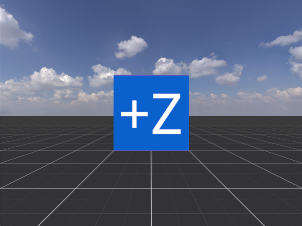
For all our troubles we get the scene:
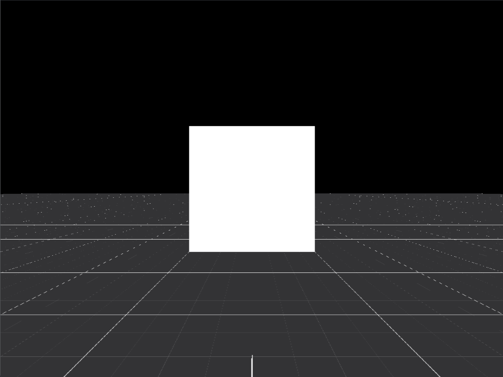
Uhh
This doesn’t look quite right. The high frequency information from the texture is lost. One thing we need to change is use a linear blending, but
that won’t solve our problems either.
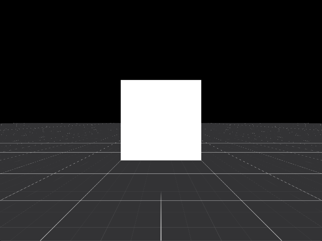
Linear interpolation
As it can be seen the lines became smoother, but the texturing still falls apart completely after a certain distance from the camera. The issue is, as with many things in graphics, the discrepancy between the sampling frequency and the frequency of the data within the texture we are sampling. In our case the texture is mostly high frequency data, in layman terms lines or hard/crisp edges. The further away the texture, the more unlikely is, that our low frequency sampling will be able to gather the requisite information. The result is that seemingly randomly the lines in the texture disappear.
For a little bit of clarification it is prudent to first understand why the term texel exists. Why is there a need to be able to differentiate between the pixel on the screen and the pixel on a texture (texel). If you just open up a texture, to be displayed by some image viewing program, what is the difference between the pixels and texels? Nothing. They are the exact same thing. As long as their ratio is 1:1, where one texel is used to create one pixels worth of information. Most often than not though, this is not the case and either more or less texels are required to produce a single pixel. Texels are the inputs, fed into a sampler to produce the output pixel. Which pixels (in this case texels) then can be used to be fed into another sampler to produce another set of pixels. The real difference between the two is, which one did you start and end with, because of this some will mix the terminology, but as you can see, in this case it is more about clarifying the usage not the concept. More about texture basics in this wonderful article: WebGPU Textures
For example in our case that white line in the middle of the screen slowly disappears, because the sampling will simply start missing the information. As the texture is sampled from further and further away, the width of the line, relative to the screen pixels will diminish, to the point that they are missed entirely. Take a look at the below example which is a closeup of the vanishing middle line in question on a pixel scale.

The green line represents, the projected pixel locations from the screen, onto the sampled texture. We are closest to the camera on the right and get farther away to the left. This line is slanted, due to the perspective projection. As an object gets further and further away from us, it appears to shrink in our view. This shrinkage, from the perspective of the texture will appear is if it was sampled by diverging lines, which originate from the camera. The yellow rectangle, is drawn between the centers of the four closest pixels that will be sampled for generating the pixel color. As it can be seen with this exaggerated example the samples drift away from the information we are seeking. In an ideal world, you would just expand the sampled area more and more, the further you get from the camera to compensate for this, but this is unfeasible in practice.
The sampling problem, lays within the domain of digital signal processing, about which whole books have been written about. However, in computer graphics tricks and shortcuts are more important if they are performant and get us 90% the way there than the actually correct solution. And it so happens there is a rather simple solution to this issue. It is called mimpmaps. The idea is staggeringly simple. We don’t want to increase the sampling rate, because that is costly. Instead we can generate smaller and smaller textures, constantly smearing the image a bit more and more. Then the further the textured point is from the camera the more smeared texture we use. In practice this means that high frequency information slowly turns into low frequency information, which can be sampled better with lower frequency.
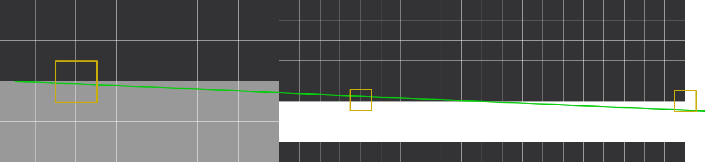
After a given distance, not the original texture is sampled, but the next mipmap level. This is blurrier, lower resolution, so the high frequency crisp white line is greyer and wider overall. In this example the line became much greyer (the effect is the result of the filtering used while downsampling, in this case a bilinear filter was used), and because the resolution is half of the original texture, each pixel takes up four times as much space in the UV coordinates. As a result the 2 pixel wide line is now 4 and the sampler manages to hit texels with the relevant information.
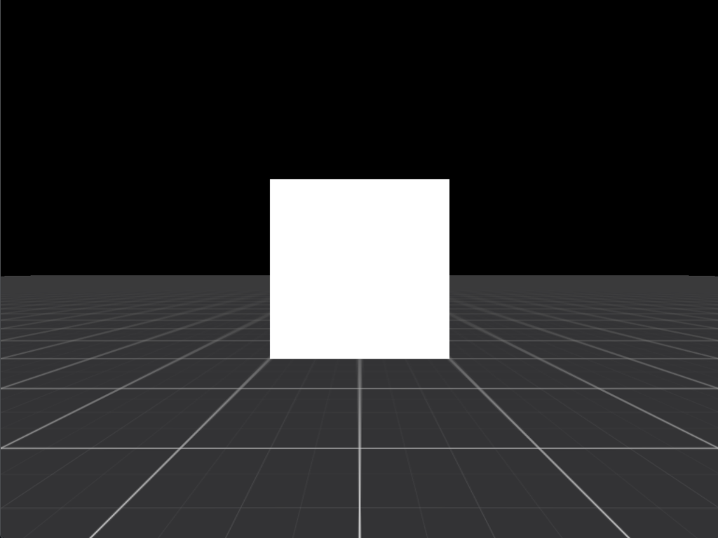
Mipmapping
If we look at the line starting from the bottom center of the screen, we can observe that as it gets further away from us, it gets wider and blurrier. Not ideal, but it is cheap to compute, and in practice it sells the illusion very well.
The cube texture
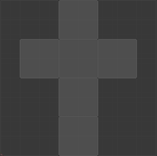
Cube UV map
If you have heard about textures before you have probably heard about UV maps/UV wrapping. Most likely you have seen one for a cube already which looks like the one above. This UV map represents where the faces of the cube would be on the texture. Notice that this is a bit wasteful though as most of the texture space is not used for the cube. About half of the whole texture is wasted.
It works of course and probably very useful while prototyping given that Blender can generate these for you. We will be doing it a bit differently by using texture atlases. Don’t be alarmed, a texture atlas is nothing but a texture, into which other smaller textures have been aggregated together.
Cube texture
When we map it onto our cube we get:
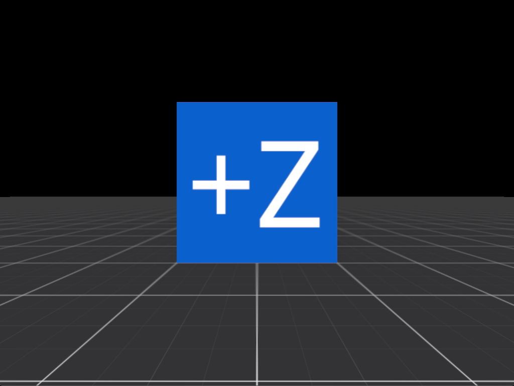
Textured cube
Which is good, but unfortunately not perfect. As described before mipmaps are necessary for any half decent texture sampling, but this also causes an issue.
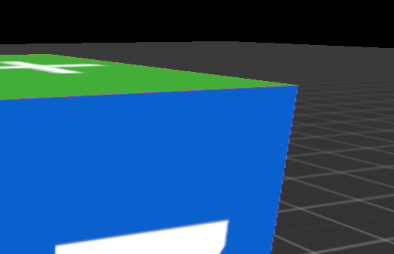
Atlas mipmap error
Because all the textures are merged into one atlas, when the mipmaps are generated they will get mixed together along the boundaries, not to mention the sample on the edges will sample into the neighbours as well. Which can lead to all kind of unwanted artifacts like the one above. The red pixels are blended into the edges of the blue and green sides.
There are ways of mitigating this, for example described in Texture atlases, wrapping and mip mapping, but for the time being such optimizations will be omitted. Our goal for now is to have the same scene as in the Godot example, which exhibits the exact same behaviour.
The Skybox
First it is best to clean up some definitions. Especially if one is new to these technologies. It is very confusing how they are mixed up left and right.
HDR, HDRI definitions
Kloofendal 48d Partly Cloudy (Pure Sky) is an image created using HDRI (High dynamic range imaging). It uses HDR (High dynamic range) to more naturally capture the wildly differing luminosity values in a scene. It is not HDR, it uses HDR (high dynamic range) instead of SDR (standard dynamic range). HDRI is the technology/methotology for capturing it (How to Create High Quality HDR Environments if you want to read more). There is no correct way to referring to their type, in leu of a proper one, often their extension is used which is either .HDR or .EXR, or this mouthful appears HDRI image (high dynamic range imaging image). The situation is a tad bit unfortunate, but it is what it is.
Another misnomer is that Skybox-es are often just equated with an HDRI image. Skyboxes often use HDRI images as textures, but any other object could use an HDRI image as well. It is simply more prevalent that the skybox is an HDRI image, because that alone can help light the scene appropriately.
Skybox implementation
There are two ways of implementing a skybox I have found so far.
Either using cubemaps or a single image using equirectangular projection. They are rather similar in their basic concept. Take the camera, project a number of rays from the eye through the center of each pixel on the Z near-plane, find the direction of these rays, then sample the texture that has been conveniently placed in model space using these directions.
Here is where we can again be grateful for the absolute brilliance of the people coming before us and marvel at the elegance by which this issue has been solved. In practice we don’t project any rays at all, but the result will be exactly the same.
Equirectangular projection
Our chosen skybox texture Kloofendal 48d Partly Cloudy (Pure Sky) is an HDRI image, produced using equirectangular projection.
Equirectangular projection
When first seeing such an image it is a bit difficult to understand what is that you are actually seeing, it looks a bit warped and just wrong. Even though you have seen such projections before if you have seen a map of Earth. Chances are, it was made using equirectangular projection. The picture of Earth doesn’t bother you, because while it does not represent reality, it is likely the only projection you have seen of it, so it appears correct by default. The projection itself is heavily distorted though. Take Greenland for example. On an equirectangular projection it looks as big the whole of North America, but its actual size is closer to the size of just Mexico. The projection will distort more and more towards the top and bottom of the projection. This is why this sky texture feels wrong. While you have seen many maps of Earth with its warped appearance and have gotten used to it, you have seen much more of the sky, without ever seeing such distortions.
Equrectangular projection describes the math behind the transformation.
Conceptually it is even simpler. Imagine there is a unit sphere centered at origo, where a camera is located at as well.
This camera rotates clockwise on the Y axis (or an axis of you choosing really) and scans whatever it sees, through the points of the unit sphere
and write it onto a 2D texture. During this scanning it always scans exactly π radians (180 degrees) vertically and 2*π radians (360 degrees)
horizontally. Producing an image which is 2*π wide and π tall. In other words twice as wide as it is tall, 2:1. (Apparently there are equirectangular
projections that only use half of the vertical resolution, resulting in a ratio of 4:1.)
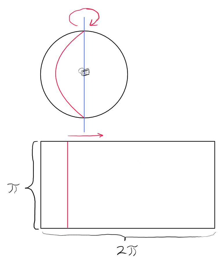
Sphere-Plane
Such images seem to be a good candidate for a skymaps/environmental maps as they encode into a single texture the whole range of surrounding visuals. This is why I would have preferred to use one as it is, but after the curveballs coming from just reading a .PNG image, it seemed to make more sense not to try and battle the hdr file formats .HDR or .EXR. Not to mention the challenges that may arise from having to handle the extended brightness ranges encoded in such an image. For these reasons, it was decided that instead an older technology of cubemaps will be used.
Skybox using a cubemap
A cubemap is nothing really just a simple axis aligned cube, that has been textured according to the requirements of our graphics API. In our case WebGPU, defines the requirements on a cubemap texture like so:
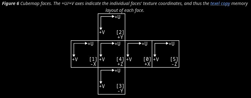
Cubemap faces
Which means that it needs exactly six textures of the same width and height in the order for the cube’s sides. In this case: +X, -X, +Y, -Y, +Z, -Z. That is a 2D array texture. This is not a 3D texture, even though we have a 3rd dimension. These are separate textures, that can be simply sampled by a vector directly, due to the built in hardware support. Also do not confuse it with the UV map of a cube, shown before. That is a method for wrapping a single texture onto a cube, while a “cubemap” is a way of texturing each individual face of the cube with a separate texture.
Using the tool panorama-to-cubemap we could turn our EXR equirectangular skymap texture into a cubemap:
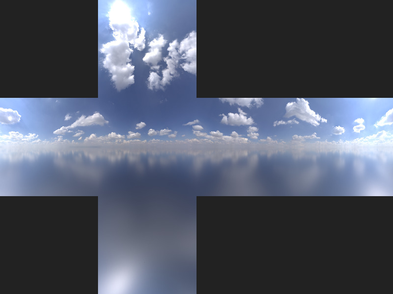
Sky cubemap
Notice that if you were to fold up the cube map, it would would look like and be oriented exactly the same as the cube in our scene. +Z facing the camera, +X going right and +Y up. The right-handed Y up coordinate system, with the standard camera direction looking down into the -Z direction.
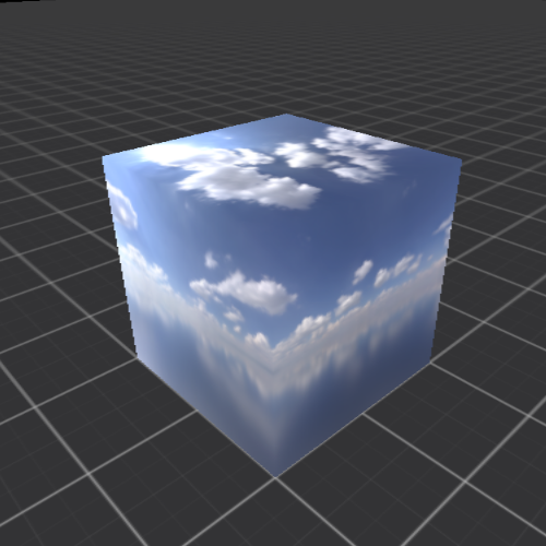
On the cube
This could be our skybox looked at from the outside, but it is not. You would have to be an extremely vigilant reader to notice that the clouds don’t appear in the order they should. The source of the confusion is orientation. The HDRI image we use as a skybox was taken as a sequence of pictures sampling the space around it. It was looking at the scene from the inside outward. The orientation of the cubemap textures expects outside in perspective. This will result in the inversion of the coordinate system. In our case we used a right handed Y up coordinate system for the world and we will need a left handed Y up coordinate system for sampling the cubemap.
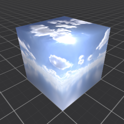
Inverted handedness
This may still be rather confusing to understand, unless you have very good spatial reasoning abilities. For one I do not, and was thinking of a way of trying to explain it properly why the inversion needs to happen, but alas, the problems true understanding is simply beyond me.
Looking at the skybox from the outside is nice and all, but what we really need is to ensure that it will be everywhere around us, always in the proper orientation.
The shader code for this is less than barely 50 lines of actual code: skybox.wgsl. What it does is very simple and beautiful. Firstly, it ensures that the skybox always appears behind everything. It does this by generating a triangle which completely covers the whole viewing area. This triangle is perpendicular to the viewing direction and is placed right at the farthest end of the normalized device coordinate space. In case of WebGPU, this will be at Z = 1.
Now it needs to sample the skybox in the appropriate orientation. From the previous step, we will have vectors <X, Y, 1> where both X and Y, can
range between [-1.0, 1.0].
If we create a view projection matrix that does not contain the translation of the camera, we will have a transformation that takes the world space,
rotates it around the origo and then projects it, arriving in at the normalized device coordinates.
What we want is to go into the opposite direction. We want to know that from our normalized device coordinates, in what direction each fragment would
be in world space. This is simply the inverse of this modified view projection matrix. By applying it, normalizing the resulting vectors, we can now
just simply sample the cubemap textures as before.
Then if we further restrict the draw call for the skybox to be the only call that can write to depth of one, there can never be anything that can appear behind the skybox. As everything else can only occupy depths of <1.0.
It is truly amazing how much a little linear algebra can accomplish.
Engine state
Putting all that behind us, we have arrived at the current engine state, achieving our goal for this iteration!
Engine state
If we compare it with the Godot based reference:
Godot reference
We can see that the two are nearly identical. There are three differences that stand out. Godot manages to have a better resolution for the cube texture, while also avoiding most noises from the texture atlas mipmap artifacts. Lastly there is some kind of “fade out”/“red shifting” effect for the plane texture in the Godot representation. The closer the horizon, the redder the plane texture seems. Not sure why this may be, maybe missed some flag or some such while writing the shader for Godot.
Code available at: v0.2 <- I know, we jumped from v0.01 to v0.2, but it made more sense to do this correction now, so that part_1, part_2 .. part_x can nicely align with v0.x tags.
Reference implementation done in Godot: v0.2
FPS counter
In the previous chapter we had the following FPS metrics:
develop build
Avg. FPS: 2743.96
1% low: 1985.52
0.1% low: 1391.16
release build
Avg. FPS: 11373.37
1% low: 8939.11
0.1% low: 8312.07
Now we have:
develop build
Avg. FPS: 2547.60
1% low: 1929.50
0.1% low: 1263.82
release build
Avg. FPS: 10790.21
1% low: 6418.93
0.1% low: 2536.53
Of course the metrics fluctuate somewhat and the above measurements are just a single snapshot, we can see that about ~200 FPS was lost in develop and ~600 FPS in release build.
Not sure what the drop means, not sure the measurement is meaningful, none the less here it is.