While one can theoretically construct some assets within a game engine itself, apart from the simplest cases this is wildly impractical. Managing the additional UV maps, normal maps, texture generation, not to mention any animation is just a set of problems that need to be solved. Putting the mesh itself together alone is a complex enough problem that whole software families have been written around it. It suffices to say, there should be no good reason for adding direct support for these within the engine itself. Simply use existing tools, generate some supported formats and import them into the engine and our problems are solved.
Now what should we support? Ideally something that can handle everything. For reference, what types of Imports & Exports does Blender support?
- Alembic - (Open source) Animated meshes stored with baked geometric results. It does not store any rigs or physics related data for reproducing the animation, only the resulting animation itself.
- BVH - BioVision Motion Capture data. Hierarchical data and its animation.
- Universal Scene Descriptor - USD is for storing whole hierarchical scenes containing cameras, meshes, lights, materials, etc..
- Stanford PLY - PLY can store mesh data, some color properties, but does not store any transformation or scene related hierarchical data.
- STL - STL only seems to contain, triangulated mesh data. No color, no materials, just the triangles and their normal.
- FBX - FBX is an Autodesk format that handles complex scene data, with animations.
- glTF - glTF is a Royalty-free specification by Khronos) for storing meshes, materials, cameras, textures, animations.
- Wavefront - Wavefront OBJ files are for storing basic geometric data and basic material properties.
And surely there are many more formats out there in the wild, but for now this list is detailed enough. As a start, something simple should be
supported, without any complex machinery like scenes and animation. That narrows it down to PLY, STL and Wavefront OBJ.
PLY and STL seem to be a bit restrictive. PLY can only contain exactly one object, and STL can only contain mesh data.
Wavefront OBJ seems to be the winner. It has a decent specification thanks to Paul Bourke it is simple,
supports more then the other two and can also handles basic material properties with the additional .mtl files.
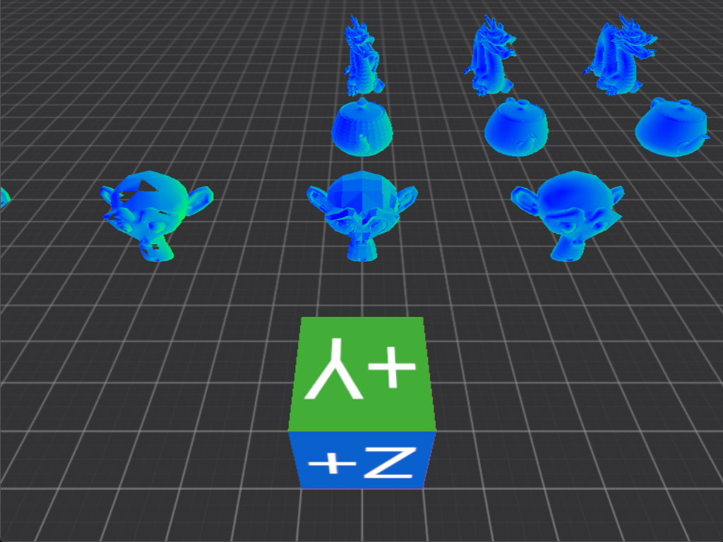
With all those decisions out of the way, lets see our reference scene.
The monkey, dragon and the teapot (walk into a bar)
The scene targeted for this chapter
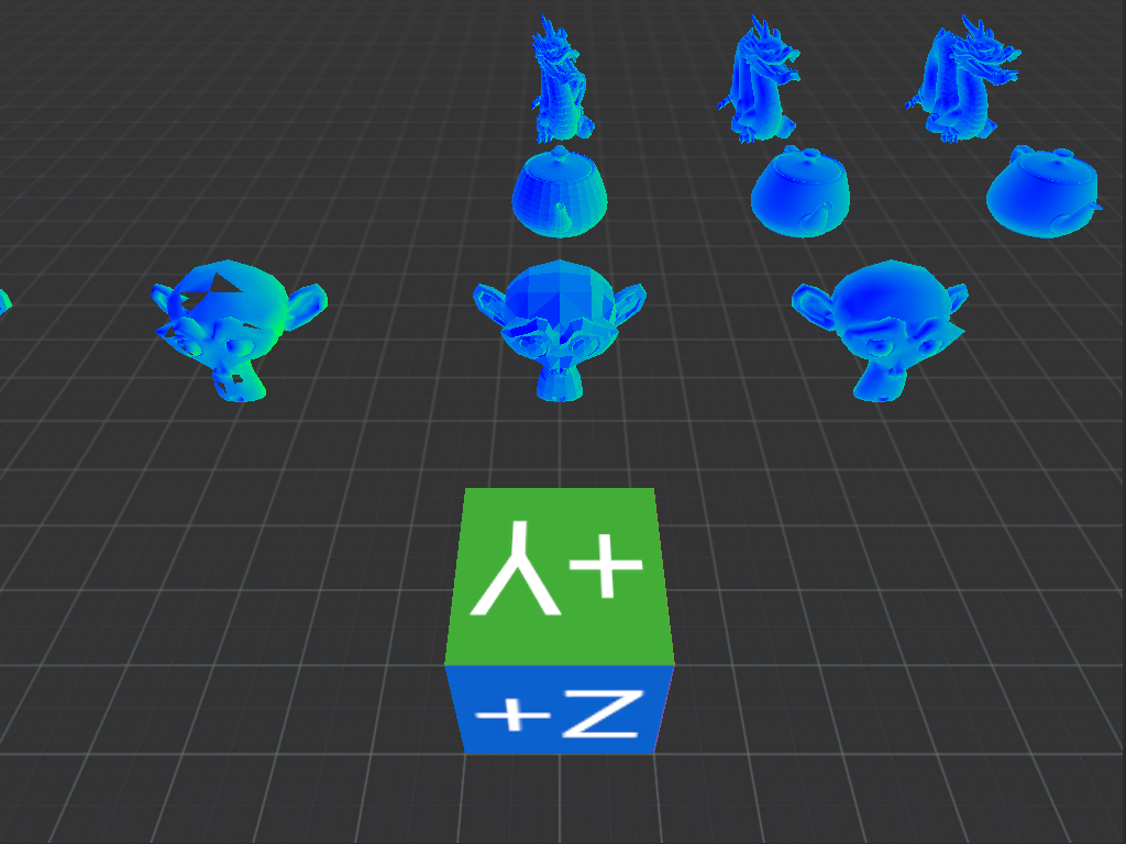
Reference scene
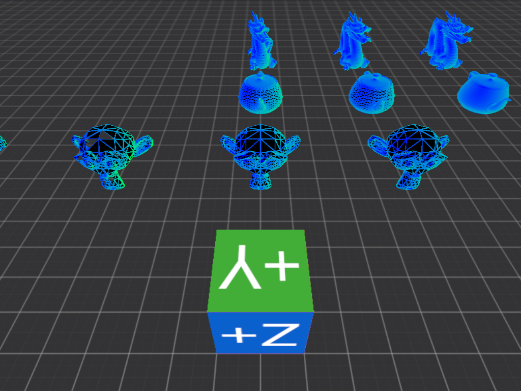
and rendered using wireframes
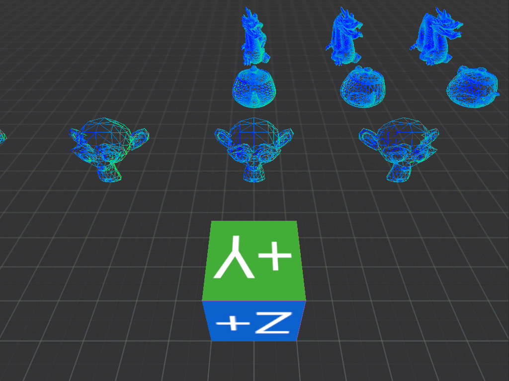
Wireframe reference scene
It should be noted that our wireframe scene will be different from the one in Godot. Simply because we will not implement any sort of LOD (level of detail) optimization for the meshes. This is a similar idea to mipmaps. The further something is, the crappier it can look and nobody will notice it while performance can increase drastically. Godot internally generates the different levels of detail from a single mesh as it is being imported. These types of algorithms are not in the scope of this post. Like scene handling, and editor gizmos, we will handle these when they become a necessity. For this simple scene they shouldn’t be, even though collectively this will be about a million triangles on the screen.
The three models on display are somewhat legendary in the graphics community. Suzanne is the monkey, built into Blender. The teapot is the 2025 - Cem Yuksel version of the Utah Teapot, which has been around in some for or another since 1975. The dragon is a 3D scan from the The Stanford 3D Scanning Repository.
Each mesh is imported multiple times for demonstrating the difference between low/high triangle counts and flat/smooth shading.
Looking down the center and going right:
- Suzanne: flat shading 967 triangles, smooth shading 967 triangles
- Teapot: flat shading 7k triangles, smooth shading 7k triangles, flat shading 116k triangles
- Dragon: flat shading 17k triangles, smooth shading 17k triangles, smooth shading 700k triangles
Additionally Suzanne is included twice more to the left with various normals flipped on the mesh for introducing artifacts as well. Both of these models have 967 triangles, one is smooth the other flat shaded. These erroneous normals make them appear incorrect in the reference scene. Engines “cull” (discards) all triangles from rendering that are not visible from their front. A triangle is considered to be viewed from the front if their normals are pointing towards the camera.
Precursor to a debug shader
As the feature set of the engine grows, it is increasingly more important to have sufficient debugging capabilities. One of them is a simple shader that can color the object based on its normals orientation. How this should work, and not be entirely boring or annoying to look at is unclear. In Blender and Godot they simply shade the front face of the triangle gray and the backface a darker gray (while also providing a myriad of other debug shader options as well). To me this doesn’t necessarily highlight any potential issues well enough. What would be ideal is to color each triangle with some pleasing tones, that are simple enough to read, but aren’t annoying. Furthermore we should be able to tell for each face if all its normals are pointing in the same way or not, by highlighting this difference. The human perception is most reactive to the red, green and blue color triplet. Red is a bit too harsh, so blue and green will be the base colors. Red will be mixed in to highlight other inconsistencies. Lastly the shader should track the camera and the angle it is looking at the object and shade appropriately. Hopefully this will lead to some, relatively pleasing results that also highlight any errors with the meshes.
As a first step though, we will do something simpler. Put a simple directional light in world space. Color the faces bluer the closer their normals align with the inverse of the light direction, and bluer otherwise. This way as a start we don’t have to track the camera, the “light” always stays in the same place allowing us to observe the coloring scheme from all angles. In the next chapter then we can finish the desired implementation.
shader_type spatial;

// turn on wireframe by adding "wireframe"
render_mode unshaded, skip_vertex_transform, wireframe;

const vec3 world_light_direction = normalize(vec3(1.0, -1.0, -1.0));

vec3 srgb_to_linear(vec3 srgb_color) {
	vec3 above = pow((srgb_color + vec3(0.055)) / vec3(1.055), vec3(2.4));
	vec3 below = srgb_color / vec3(12.92);
	return mix(above, below, lessThanEqual(srgb_color, vec3(0.04045)));
}

vec3 linear_to_srgb(vec3 linear_color) {
	vec3 above = (vec3(1.055) * pow(linear_color, vec3(1.0 / 2.4))) - vec3(0.055);
	vec3 below = vec3(12.92) * linear_color;
	return mix(above, below, lessThanEqual(linear_color, vec3(0.0031308)));
}

// flat means not to interpolate the value for the fragment shader
varying flat vec3 light_direction;

void vertex() {
	vec4 model_vertex_position = vec4(VERTEX, 1.0);
	NORMAL = MODELVIEW_NORMAL_MATRIX * NORMAL;
	VERTEX = (PROJECTION_MATRIX * MODELVIEW_MATRIX * model_vertex_position).xyz;
	// skip_vertex_transform disables Model and View transformations for a vertex, but
	// by setting POSITION ourselves even projection is disabled.
	// This is not necessary, but as a learning experience it is helpful to see the whole transformation
	// pipeline applied to each vertex, without it being obfuscated by some internal behavior.
	POSITION = PROJECTION_MATRIX * MODELVIEW_MATRIX * model_vertex_position;
	// The light direction only needs to transformed by the View matrix and since it it only a direction
	// only rotation is applied to it.
	light_direction = normalize((VIEW_MATRIX * vec4(world_light_direction, 0.0)).xyz);
}

void fragment() {
	vec3 normal = normalize(NORMAL);

	float similarity = (dot(-light_direction, normal) + 1.0) / 2.0;
	vec3 color = mix(vec3(0.0, 1.0, 0.0), vec3(0.0, 0.0, 1.0), similarity);
	// We are using linear values to define the green and blue colors and Godot
	// renders using linear color space, so no transformation is needed.
	ALBEDO = color;
	// In case you would like to experiment with incorrect values.
	//ALBEDO = linear_to_srgb(color);
	//ALBEDO = srgb_to_linear(color);
}
Before we continue a little sidestep.
Linear vs sRGB color space
In the previous chapter we encountered that the textures just didn’t seem to have the same color/saturation/brightness in Voxon as they did in Godot. To mitigate this we used a conversion function:
// force SRGB color <- by the way this was incorrect too. This is converting from sRGB to linear color space.
	ALBEDO = mix(pow((sample + vec3(0.055)) * (1.0 / (1.0 + 0.055)), vec3(2.4)), sample * (1.0 / 12.92), lessThan(sample,vec3(0.04045)));
The issue was that Godot expects shaders to calculate within the linear color space. Then it will apply the necessary transfer functions (in this case sRGB) before rendering the final image. When a texture sampler is constructed, by default it also expects the textures to be in linear color space. In other words when sampling the texture it won’t apply any transformations to it.
The expected pipeline would have been: read linear texel data -> calculate color with linear values -> apply sRGB transfer function (Godot)
What we did: read sRGB texel data -> calculate color values with sRGB values -> apply the inverse sRGB transfer function -> apply the sRGB transfer function (Godot)
The last step in both cases is done by Godot automatically. This is why the misused and misnamed function call seemed to solve the problem. The result was still incorrect and it would never have been correct until the calculations were moved into linear space as well. From Godot, it only needs us to either tell the sampler that it is reading an sRGB texture or supply it a texture using linear colors.
This is one of the reasons why it is usually very bad to copy code from online. The copied code does the opposite what it claimed and it didn’t even solve the problem.
Why the difference? Simply put the linear color space is used for calculations, blending, sampling etc., the color values range between 0-255. On the other hand the sRGB space is for the monitors. The legend says that CRT monitors used the sRGB transfer function given that experiments shoved that the produced colors will be perceived by the users to be close to what they represented numerically. Monitors evolved and they use different transfer functions now. Non the less, most of them, by default expect the incoming colors to be in sRGB color space, which then they internally convert using their own transfer functions. Ahhhh, the historical reasons are the best. At least it makes sense and gives backward compatibility. (By the way I have heard other legends that good quality CRT monitors now produce better quality images than most high-end monitors. Maybe this is one of the reasons why.)
Anyways the shaders now contain the linear <-> sRGB transfer functions allowing you to play around with them as well.
Importing the first .obj
As decided before the Wavefront OBJ will be used as the file format of choice. The format is ancient and many extensions have been added to it throughout the years. This complexity and the lack or original specifications, reference implementations makes it error prone in practice. The issue can be sidestepped though, if we only focus on its most basic features and ignore all the rest. In this case we only need it to be able to describe a triangulated mesh using positional/normal/uv vectors for each vertex. That is it. Everything else we can ignore. With these restrictions a ‘.obj’ file looks like this for a simple plane:
# Blender 5.1.1
# www.blender.org
o Plane
v -1.000000 0.000000 1.000000
v 1.000000 0.000000 1.000000
v -1.000000 0.000000 -1.000000
v 1.000000 0.000000 -1.000000
vn -0.0000 1.0000 -0.0000
vt 1.000000 0.000000
vt 0.000000 1.000000
vt 0.000000 0.000000
vt 1.000000 1.000000
s 0
f 2/1/1 3/2/1 1/3/1
f 2/1/1 4/4/1 3/2/1
Components:
- ‘#’ comment
- ‘o’ group name
- ‘v’ positional vector
- ‘vn’ normal vector
- ‘vt’ uv coordinate vector
- ‘f’ faces
- ’s’ smoothing group (we can ignore this)
That is all. First, all the data is specified and put into their respective buffers, then the faces index these buffers using the format vertex index/uv coordinate index/normal index. For some reason the indexes are counted from 1 instead of 0, but apart from that, this is it. (We ignore here of course that some vectors have optional components, that faces don’t have to specify everything only the position, that you can use negative indexes, that it isn’t strictly specified that every vertex has to be defined at the beginning etc..)
When we implement the parser and import Suzanne, we get this
Suzanne
What we see is Suzanne textured as the plane. This is not what we want but it is good demonstration of another problem. That of complexity. To render the plane, we needed buffers to write the vertex positions/normals/texture coordinates into. Another buffer to index these buffers. A texture, that we had to mipmap, for which we had to allocate another buffer. Then to access that texture we needed a sampler. A similar problem for rendering the cube, which also uses a different kind of texturing pattern. The skybox is completely different as well. Now we want to render without textures by using some simple shaders instead. Managing all this is rather difficult. More difficult it will get still when later on we want to actually add materials, lights, shadows etc.. Based on the combinations of the required features for rendering a given object different pipelines, shaders and configurations must be set up.
In some engines this means that they have billions of shader pipelines. All tailored for a given permutation of features. In others they have a few “ubershaders” which handle most of the possible configurations. In the earlier days the first approach was more prevalent, because the GPU was a very limited resource, it didn’t like branches too much and the register pressure was too high. To squeeze out all the performance it was more economical to generate custom setups for each task (the graphics weren’t on today’s complexity we might add). This way one could avoid writing branches, as it was known exactly what will happen, before the code was even written. Since then the GPUs have evolved a bit and are much better at branching. The graphics pipelines also got much more complex, to the point that the aforementioned possibly billions of combinations are more of a detriment than a handy optimization. With so many possibilities and switching between different executions it is extremely difficult to retain any decent cache coherency. This is truly a huge engineering problem and it is already causing problems for me. Never the less we must soldier on for a good while longer, while incrementally refactoring sections if they become very troublesome.
Implementing the “normal debug” shader precursor
After refactoring the main scene, separating out the plane and cube as the textured objects and building out a whole new pipeline for the “debug shader”, finally Suzanne should be shaded properly!
Oh no, that isn’t quite right. When the camera orbits Suzanne blue sections turn green and green sections turn blue. How can this be? Deliberately restricted the implementation of the shader to always produce the same result regardless of the cameras or the objects orientation.
Here are the relevant parts of the shader:
const world_light_direction = normalize(vec3(1.0, -1.0, -1.0));

@vertex
fn vs_main(vertex: Vertex) -> VSOutput {
    var vsOut: VSOutput;

    // Compute the vertex position in device coordinates
    vsOut.position = global.view_projection * entity.world * vertex.position;

    // Orient the normals in world space
    vsOut.normal = entity.normal * vertex.normal;
    vsOut.light_direction = normalize((global.view * vec4f(world_light_direction, 0.0)).xyz);
    // the returned vector will automatically be normalized using w
    // [x,y,z,w] => [x/w, y/w, z/w, 1]
    return vsOut;
}

@fragment
fn fs_main(vsOut: VSOutput) -> @location(0) vec4<f32> {
    // All inter-stage variables get interpolated, so they
    // have to be renormalized if necessary.
    let normal = normalize(vsOut.normal);
    let light_direction = vsOut.light_direction;

    let similarity = (dot(-light_direction, normal) + 1.0) / 2.0;

    return vec4(mix(vec3f(0.0, 1.0, 0.0), vec3f(0.0, 0.0, 1.0), similarity), 1.0);
}
We can see that it is nearly exactly the same as the Godot reference implementation. A few minor differences are observable, for example
here a view_projection * world matrix is used and in Godot a projection * modelview combination. These are the exact same thing and will result
in the combined model view projection matrix. So the code is the same, yet still behaves differently.
Hmm, what can it be. After some experimentation it turned out that if the light_direction is simply set as the world_light_direction, without
any transformations, the result will stabilize and appear as expected. Curious, curious, because that light was defined to be in world space,
so it must be transformed by the View matrix. The transformation must be applied to it, otherwise it would not be oriented in the appropriate direction.
This can be confirmed, by disabling the transformation in the Godot reference. What we will see will be the exact same issue we observe here.
By the movement of the camera the shader output changes.
So in Godot, the transformation is necessary, while for us it is actively causing the issue? Marvelous!
Maybe there is a bug in the normal matrix? How could there be? In Part 1, the normal matrix already functioned
correctly with the camera orbiting around the object. But something is clearly not rotating when it should and bamm it hit me!
My normal matrix does not contain the view matrix, so it does not correct for the movement of the camera!
If we look at the Godot version, the matrix is called MODELVIEW_NORMAL_MATRIX. It contains the model and the view transformations!
Mine only contained the model! After fixing the issue the shader behaves as expected.
Okay, but then why was it working in Part 1? Very simple, there the light, camera, vertex positions and the respective directions were
all calculated in world space (just the model matrix was applied). In this shader they were calculated in model view space.
All objects ready
Imported objects
All the target objects are imported and look as expected. After the color transfer function fixes, the colors too appear the same.
Voxon vs Godot
Let us see what happened with the framerates after adding this circa million polygons to the scene. As a reminder previously
develop build
Avg. FPS: 2547.60
1% low: 1929.50
0.1% low: 1263.82
release build
Avg. FPS: 10790.21
1% low: 6418.93
0.1% low: 2536.53
and now
develop build
Avg. FPS: 1949.03
1% low: 1849.82
0.1% low: 1816.83
release build
Avg. FPS: 4476.02
1% low: 1883.10
0.1% low: 1414.46
That is a rather big hit. In the debug build we have lost about ~600 frames on average, in the release
almost ~6000. Nearly half the frames are gone with the wind after adding only this many polygons. To be honest,
not sure how many are too many, but nowadays a million, especially on the GPU sounds like an afterthought.
This should be investigated a bit further, before additional complications are added to the engine. For once, the code wasn’t
kept too clean, secondly there are a few optimization ideas that should be put to the test.
Thus, instead of adding a wireframe rendering option, first we will break the engine and see how we can fix it.
To the limits
Currently the code was written in the simplest copy/paste way possible. Completely disregarding any performance considerations. Every mesh is loaded/uploaded to the GPU for every pipeline, all of them use separate draw calls as well.
Now that we have some meshes, which we can duplicate and position as required, the easiest way to increase the load on the GPU is to just simply render more meshes. By adding the same mesh over and over, using the same shader a specific setup is reached. One where most objects in the scene use the same mesh and the same shader. Which means that two optimization strategies can be tested one after another. Reducing the number of draw calls and then the number of polygons.
Adding the smooth shaded utah teapot with about 7k polygons, 16x16x16 = 4096 times, using up about 28'672'000 polygons, we still
hover around 90 FPS on average in release build.
Avg. FPS: 89.07
1% low: 38.90
0.1% low: 35.40
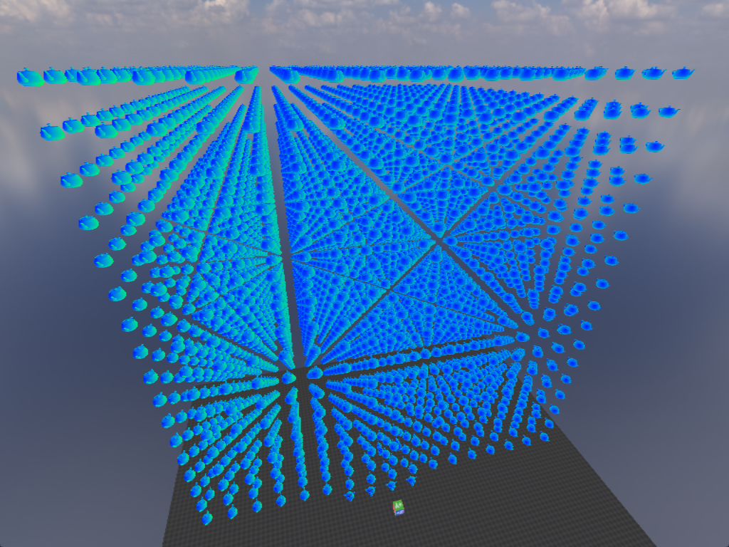
Utah cube
In fact adding more of them after about 16x16x8 didn’t seem to affect the FPS any more, even though we have no LOD or any type of
optimization on our side to speak off.
Maybe the vertex concentration is simply not high enough?
Replacing the teapot cube with the smooth shaded stanford dragon using 700k polygons in a 5*5*3 = 75 pattern, using up
52'500'000 polygons seems to do the trick. Now in release build we still get about a 100 FPS on average but the 1% lows, especially
the 0.1% lows start to tank.
Avg. FPS: 113.56
1% low: 27.00
0.1% low: 7.55
Dragon cubelike
This is getting noticeably choppier. Moreover, adding just one more layer on the Y axis makes it completely unusable.
A good candidate for observing how basic code restructuring and optimizations may affect performance.
At the moment every single object has it’s own mesh instance in memory, its own buffers allocated on the GPU. Within each render pipeline, there is a draw call for each individual object.
The stanford dragon is a very good example for the potential costs. Each 700k polygon stanford dragon uses up about 66'844'704 bytes of memory. Having 75 instances of them totals in 5'013'352'800 bytes or 5 GB of VRAM used. CPU utilization barely reaches 1% which is a bit surprising, because every render cycle all objects get their transform matrices recalculated and we have 87 objects to render. Admittedly, not that many, but still with a full running operating system and calculating multiple 4x4 matrix multiplications for 87 objects, even at 4000 FPS barely registers a 2 % load. On the other hand GPU utilization is obviously at 100% all the times. We render as many frames as it is willing, and as we see it, the CPU is not the bottleneck, so at least in this examination, just focusing on our handy dandy framerate calculator we can observe how helpful each optimization is.
The first thing we can do is instancing. From the GPUs perspective this doesn’t really mean anything. Just that
we want to execute a given draw call instance number of times. What we do with those indexes is up to us.
In this case though, the more common definition of instancing is used, which means the same mesh is drawn
instance number of times using different transformation matrices.
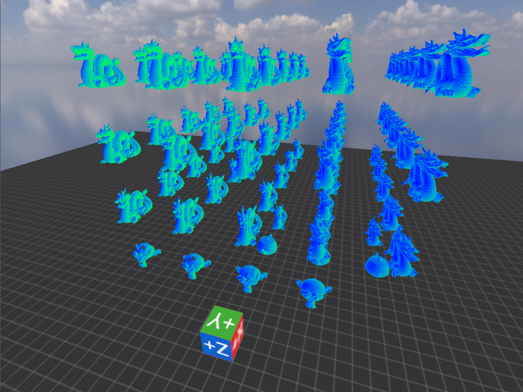
After replacing all 700k polygon stanford dragons in the scene with instanced rendering we get the following:
debug
Avg. FPS: 211.86
1% low: 89.69
0.1% low: 70.92
release
Avg. FPS: 211.86
1% low: 89.69
0.1% low: 70.92
VRAM usage is substantially reduced (5 Gb -> ~6 MB) and performance became much more stable. Average FPS is good to be high, but more important is that 1% and 0.1% lows don’t drop now below 60. That means no hitching at all. Keep in mind, only the number of draw calls changed. The same number of polygons, the same shaders, just the code was structured in such a way that the GPU had to be asked only once to draw the all 75 dragons. Already a massive improvement.
If we also replace all 700k poly stanford dragons with the lower resolution 17k polygon version, we would get:
debug
Avg. FPS: 1262.98
1% low: 1214.46
0.1% low: 1202.26
relese
Avg. FPS: 5417.23
1% low: 1818.27
0.1% low: 1775.12
Replacing 52'500'000 polygons with only 75 * 17'000 = 1'250'000, a 42x reduction, resulted in a worst case performance gain of 25x. This is why Godot immediately generates LOD levels for each mesh. The performance gains can be enormous, without much degradation in detail.
Just out of curiosity how does Godot perform? Using Vulkan 1.4.335, without the 75 extra dragons the editor reports ~2000 FPS. If all 75 dragons are present it still manages to crank out ~670 FPS. If on the other hand we completely turn of Mesh LOD optimization, the framerate drops to about 125 FPS. Now this is a much fairer comparison to Voxon, as we don’t have Mesh LOD at all. When the project is built, with all its optimizations in debug/release it will run at about 2200/2600 FPS. Pretty impressive to be honest. Didn’t expect it to be so performant.
The lesson seems to be very simple. More draw calls is bad. More polygons, even worse.
Wireframes
Back to wireframes. Rendering a wireframe representation of a given mesh is both simple and surprisingly difficult.
Using barycentric coordinates
Firstly we could do it using barycentric coordinates.
This would lead to a very simple implementation where the vertex shader generates a vector for each vertex based on its index.
This vector, the barycentric coordinate, will be calculated like so:
vsOut.barycentric_coordinate = vec3f(0);
vsOut.barycentric_coordinate[vertex.vertex_index % 3] = 1.0;
In other words each vertex will become one of <1.0, 0.0, 0.0>, <0.0, 1.0, 0.0>, <0.0, 0.0, 1.0>, which is analogous to the
unit weights assigned to each vertex in the barycentric coordinate system. Then due to the linear interpolation by the
pixel/fragment shader stage we would have the actual barycentric coordinate calculated for each fragment for basically free.
Then finally we could pick the smallest weight (the smallest distance to an edge), check if it is above or below a threshold
and set the transparency of the fragment to 0.0 or 1.0. Above the threshold it should be fully transparent, below, fully opaque.
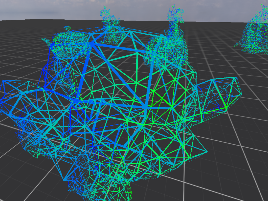
Barycentric wireframe
There is a problem though. Chiefly that we can’t define the width of the lines in pixels or meters. Nor are they of the same width using the same threshold value, in this case 0.03. To see a bit easier, the same wireframe, but only the front faces are visible:
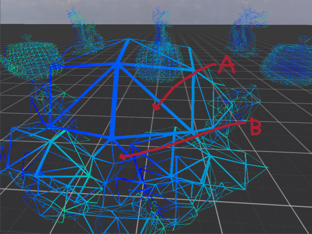
Front faces Barycentric wireframe
Take a look at triangle A and B. Observe that A has wider outlines than B. The reason is simple. Barycentric coordinates
don’t take account for the size of the triangle in screen space. Thus a triangle that takes up more screen space will have
proportionally wider lines than a smaller one. The effect is initially subtle, but becomes rather annoying after observing it.
There are sources out there where they apply additional transformations to the barycentric coordinates within the fragment shader and calculate a so called edge factor:
fn edge_factor(barycentric_coordinate: vec3f) -> f32 {
    let d = fwidth(barycentric_coordinate);
    let aliased = smoothstep(vec3f(0.0), d * line_width, barycentric_coordinate);
    return min(min(aliased.x, aliased.y), aliased.z);
}
First of all what are we doing?
fwidth will calculate the partial derivative
of the vertex coordinates in regards to the x and y window coordinates. Quite frankly, not sure what that exactly means and there
is precious little documentation about it. The smoothstep
is simply interpolates between two values in a non-linear fashion. This in practice means
that there won’t be a hard transition between the two values, but a soft one, in other words, antialiasing is applied.
Last line is just as before, get the closest edge ‘distance’.
This doesn’t work either. It alleviates the scaling problem to some extent but it doesn’t solve it. Why?
We are still working within a barycentric system which is disconnected from the screen space. line_width is in incomprehensible units, because
all the other values are in incomprehensible units as well. To demonstrate why this version doesn’t work either, here is a comparison between it
and how the same scene would look in Godot.
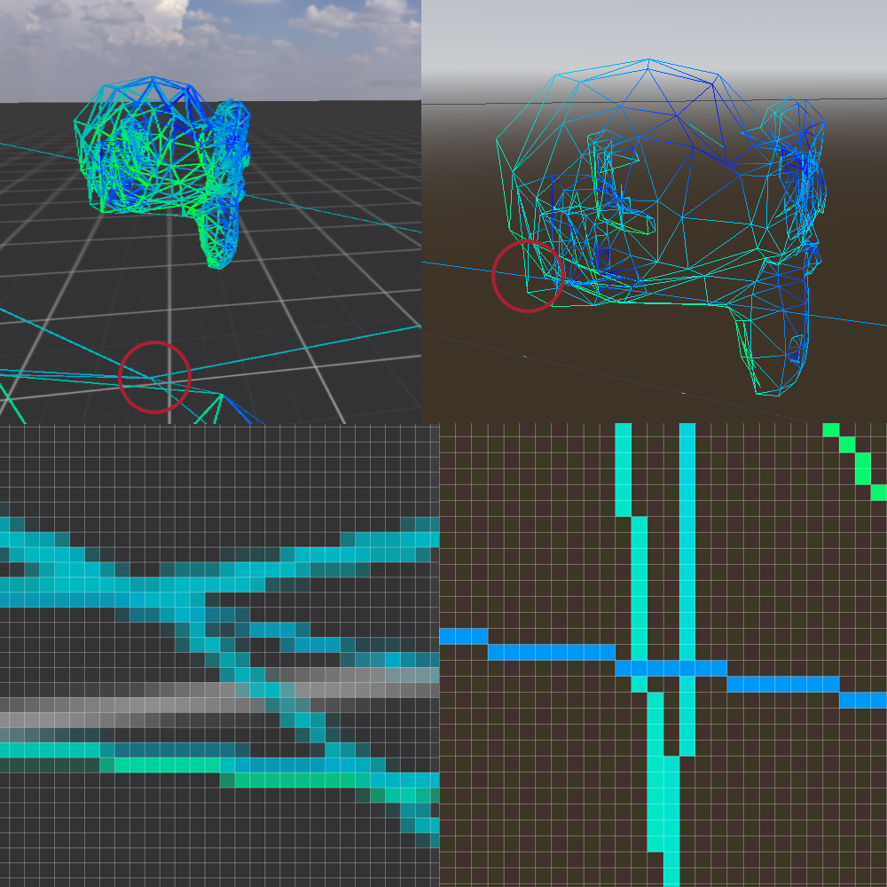
Wireframe comparison
On the left our implementation using edge_factor to generate antialiased wireframe lines, on the left Godot.
Notice how in Godot, every line is exactly one pixel wide, regardless it’s distance from the camera. While on the left lines even
close to the camera have differing widths, which is not just the result of the antialiasing step. Worse, lines further away will appear
even wider. The effect is even more jarring if we navigate the 3D space.
A better approach is needed. One where line widths can be set according to some human compatible metric and aren’t affected by the size of each triangle or by projection.
Calculating distance to nearest edge
Thankfully, like with many things in life, this problem has been solved already. It is called Single-pass Wireframe Rendering, with some more detailed description in Solid Wireframe. The idea is really simple. To render a wireframe with a configurable line width that stays stable across the whole screen we simply have to calculate the line width in screen space.
In the vertex shader transform every vertex as you normally would, then in the geometry shader (when you are working with whole polygons), calculate
the triangle’s altitudes for each polygon vertex in screen space. Emit these, with linear interpolation and by the fragment shader this vector will contain
the fragments distance from all polygon edges in screen space. At this point a simple comparison is the only thing necessary to know if we are
within x pixels of any edge. A beautiful solution!
Had a little problem though. WebGPU lacks a geometry shader stage. No easy calculations for me. Nevertheless, with a little calculation wastage it can be done within the vertex shader itself.
struct VSOutput {
    // The pixel position on the screen.
    @builtin(position) position: vec4f,
    // Will be interpolated and have to renormalized.
    @location(0) normal: vec3f,
    @location(1) @interpolate(flat) light_direction: vec3f,
    @location(2) @interpolate(linear, center) altitude: vec3f,
};

const world_light_direction = normalize(vec3(1.0, -1.0, -1.0));
// hard coding it for now
const WIDTH = f32(1024);
const HEIGHT = f32(768);

@vertex
fn vs_main(vertex_input: VertexInput) -> VSOutput {
    var vsOut: VSOutput;

    let face_start_index = entity.vertex_index_offset + ((vertex_input.vertex_index / 3) * 3);
    var vertices: array<vec4<f32>, 3>;
    // transform all vertices into clip space
    vertices[0] = global.view_projection * entity.world * vertex_data[face_start_index].position;
    vertices[1] = global.view_projection * entity.world * vertex_data[face_start_index + 1].position;
    vertices[2] = global.view_projection * entity.world * vertex_data[face_start_index + 2].position;
    // transform all vertices into NDC
    vertices[0] = vertices[0] / vertices[0].w;
    vertices[1] = vertices[1] / vertices[1].w;
    vertices[2] = vertices[2] / vertices[2].w;
    // transform all vertices into screen space
    var screen_space_vertices: array<vec2<f32>, 3>;
    screen_space_vertices[0] = (vertices[0].xy + vec2f(1.0)) * vec2f(0.5 * WIDTH, -0.5 * HEIGHT);
    screen_space_vertices[1] = (vertices[1].xy + vec2f(1.0)) * vec2f(0.5 * WIDTH, -0.5 * HEIGHT);
    screen_space_vertices[2] = (vertices[2].xy + vec2f(1.0)) * vec2f(0.5 * WIDTH, -0.5 * HEIGHT);
    let a = screen_space_vertices[2] - screen_space_vertices[1];
    let b = screen_space_vertices[2] - screen_space_vertices[0];
    let c = screen_space_vertices[1] - screen_space_vertices[0];
    // calculate triangle area using https://en.wikipedia.org/wiki/Exterior_algebra
    // we omit the division by two, because we would have to multiply by 2 when
    // calculating the altitudes
    let face_area: f32 = abs(b.x*c.y - b.y*c.x);
    // calculate screen space altitude for the triangle sides
    var screen_space_altitudes: array<vec3<f32>, 3>;
    screen_space_altitudes[0] = vec3<f32>(face_area / length(a), 0.0, 0.0);
    screen_space_altitudes[1] = vec3<f32>(0.0, face_area / length(b), 0.0);
    screen_space_altitudes[2] = vec3<f32>(0.0, 0.0, face_area / length(c));

    let vertex = vertex_data[entity.vertex_index_offset + vertex_input.vertex_index];
    // Compute the vertex position in device coordinates
    vsOut.position = global.view_projection * entity.world * vertex.position;
    // Orient the normals in world space
    vsOut.normal = entity.normal * vertex.normal;
    vsOut.light_direction = normalize((global.view * vec4f(world_light_direction, 0.0)).xyz);
    vsOut.altitude = screen_space_altitudes[vertex_input.vertex_index % 3];
    // the returned vector will automatically be normalized using w
    // [x,y,z,w] => [x/w, y/w, z/w, 1]
    return vsOut;
}
As it can be seen for every single vertex we recalculate the values for every other vertex within the triangle. Could have created another set of buffers and precalculated this with a compute shader, but the additional complexity was deemed undesirable while just trying out this algorithm.
All that said, this is how it looks:
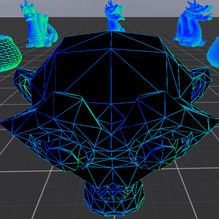
Solid wireframe
I know I know, it is not transparent as set out in the original goals. The reason is that it seems to be rather difficult to render transparency properly. Especially if you have multiple transparent object in the scene through which you could see the others. It requires rendering the objects from furthest to closest, after everything non transparent has already been rendered. Too much hassle for too little gain. As it can be seen the stanford dragons already have so many polygons, that at this distance they almost look completely solid. If they were transparent, even from close up it is rather difficult to see what is happening.
Regardless, the point of this image is to show that we have fixed the issue of relative line widths and now both smaller and larger triangles have lines of the same width. Two problems remained. For some reason my lines have some antialiasing on them even though no MSAA or prefiltering is used. Could not figure out where this smoothing is coming from. It has to be the window manager or some other default setting from WebGPU.
The other problem is that I haven’t finished implementing the whole Solid Wireframe. The rest of it gets a bit more involved and didn’t seem necessary at this time, given the issue only rears its head if a polygon is not entirely in frame, and one of its vertices is close to the camera or right behind it. In these instance screen space projection falls apart and distance measurements become irrelevant.
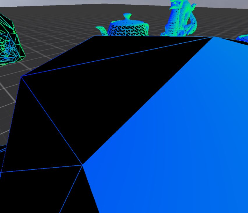
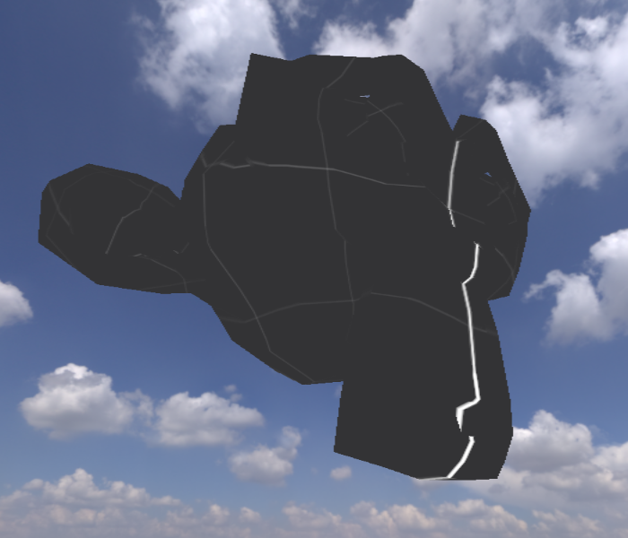
Solid wireframe bug
The bug appears as the sudden full coloring of an affected triangle. Once again, this is just my laziness, the algorithm outlined in the paper handles this as well.
Engine state
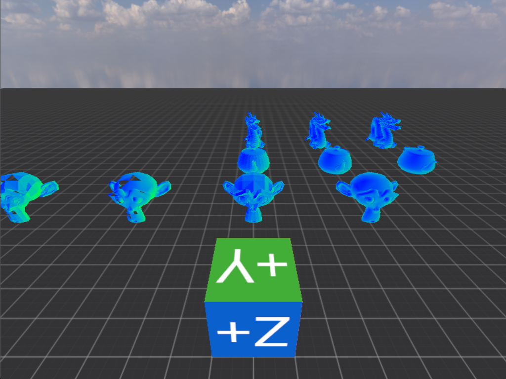
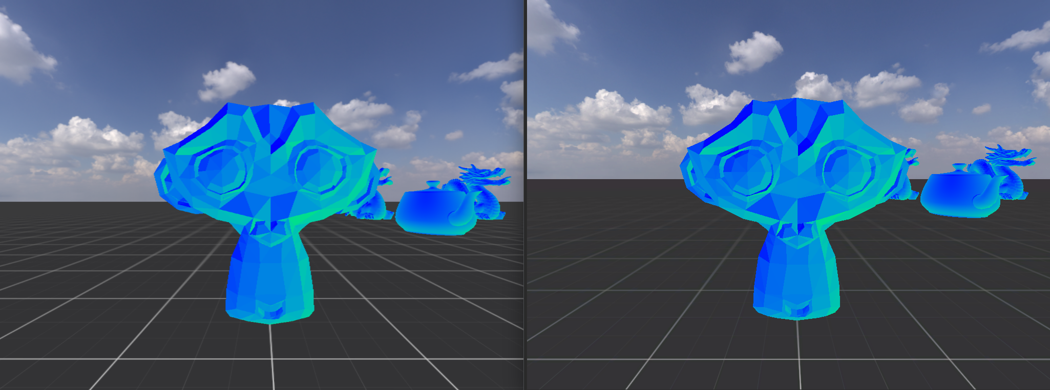
After all that trouble, let’s compare with the reference scene. First the Voxon output, then the reference.
Voxon scene
Reference scene
Voxon wireframe scene
Wireframe reference scene
Every object location, transformation is using the exact same parameters as in Godot. The camera location is the same, same FOV of 75 degrees as well. The only difference is that in Godot the camera is pitched -45 degrees, while in Voxon only -44.759. Not entirely sure why this difference is necessary and we can see the setup between the two is not exactly the same, but this was the closest I could get them. At -45 degrees with Voxon, the line of dradons in the back would barely be in view.
Code available at: v0.3
Reference implementation done in Godot: v0.3
FPS counter
In the previous chapter we had the following FPS metrics:
develop build
Avg. FPS: 2547.60
1% low: 1929.50
0.1% low: 1263.82
release build
Avg. FPS: 10790.21
1% low: 6418.93
0.1% low: 2536.53
Now we have:
develop build
Avg. FPS: 1957.49
1% low: 1850.92
0.1% low: 1785.03
release build
Avg. FPS: 4728.06
1% low: 1564.94
0.1% low: 1539.11
Even only a million polygons is a decent hit to performance. In the next chapter we will refactor the structures substantially, which is likely to provide us with even mooarrr performance!